Numerical Analysis: 2012

Saturday, May 5, 2012

12.11

A peristaltic pump delivers a unit flow (Q1) of a highly viscous fluid.The network is depicted in Fig. P12.11. Every pipe section has the same length a diameter. The mass and mechanical energy balance can be simplified to obtain the flows in every pipe. Solve the following system of equations to obtain the flow in every stream.

Q3 + 2Q4 - 2Q2 = 0
Q5 + 2Q6 - 2Q4 = 0
3Q7 - 2Q6 = 0
Q1 = Q2 + Q3 == % -Q1 + Q2 + Q3 = 0
Q3 = Q4 + Q5 == % -Q3 + Q4 + Q5 = 0
Q5 = Q6 + Q7 == % -Q5 + Q6 + Q7 = 0

Matlab:

% 7 6 5 4 3 2 1

A = [ ...

0 0 0 2 1 -2 0;

0 2 1 -2 0 0 0;

3 -2 0 0 0 0 0;

0 0 0 0 1 1 -1;

0 0 1 1 -1 0 0;

1 1 -1 0 0 0 0;

0 0 0 0 0 0 1 ];

syms Q1 ;

B = [0; 0; 0; 0; 0; 0; Q1];

display(A)

display(B)

x = A\B;

display(x)

A =

0 0 0 2 1 -2 0
0 2 1 -2 0 0 0
3 -2 0 0 0 0 0
0 0 0 0 1 1 -1
0 0 1 1 -1 0 0
1 1 -1 0 0 0 0
0 0 0 0 0 0 1

B =

0
0
0
0
0
0
Q1

x =

Q7= (8*Q1)/85
Q6= (12*Q1)/85
Q5= (4*Q1)/17
Q4= (22*Q1)/85
Q3= (42*Q1)/85
Q2= (43*Q1)/85
Q1

Saturday, April 28, 2012

11.27

As described in Sec. PT3.1.2, linear algebraic equations can arise in the solution of differential equations. For example, the following differential equation results from a steady state mass balance for a chemical in a one-dimensional canal.

0 = D * d^c/dx^2 - U * dc/dx - kc

where c = concentration, t = time, x = distance, D = diffusion coefficient, U = fluid velocity, and k = a first-order decay rate.Convert this differential equation to an equivalent system of simultaneous algebraic equations. Given D = 2, U = 1, k = .2, c(0) = 80 and c(10) = 20, solve these equations from x = 0 to 10 with delta_x = 2, and develop a plot of concentration versus distance.

derivatives

dc_dx = (c(x + dx) - c(x)) ./ dx ;

d2c_dx2 = (c(x + dx) - 2 * c(x) +c(x - dx)) ./ dx^2;

delta x = 1

dc_dx = (c(x + dx) - c(x)) ;

d2c_dx2 = (c(x + dx) - 2 * c(x) +c(x - dx));

0 = D * c(x + dx) - 2 * c(x) + c(x - dx) - U * (c(x + dx) - c(x)

c1 0 = D*c(2) - 2*D*c(1)+ D*c(0) - U*c(2) + U * c(1)

c2 0 = D*c(3) - 2*D*c(2)+ D*c(1) - U*c(3) + U * c(2)

c3 0 = D*c(4) - 2*D*c(3)+ D*c(2) - U*c(4) + U * c(3)

c4 0 = D*c(5) - 2*D*c(4)+ D*c(3) - U*c(5) + U * c(4)

c5 0 = D*c(6) - 2*D*c(5)+ D*c(4) - U*c(6) + U * c(5)

c6 0 = D*c(7) - 2*D*c(6)+ D*c(5) - U*c(7) + U * c(6)

c7 0 = D*c(8) - 2*D*c(7)+ D*c(6) - U*c(8) + U * c(7)

c8 0 = D*c(9) - 2*D*c(8)+ D*c(7) - U*c(9) + U * c(8)

c9 0 = D*c(10) - 2*D*c(9)+ D*c(8) - U*c(10) + U * c(9)

c1 0 = D*c(2) - U*c(2) + U * c(1) - 2*D*c(1) + D*c(0)

c2 0 = D*c(3) - U*c(3) + U * c(2) - 2*D*c(2) + D*c(1)

c3 0 = D*c(4) - U*c(4) + U * c(3) - 2*D*c(3) + D*c(2)

c4 0 = D*c(5) - U*c(5) + U * c(4) - 2*D*c(4) + D*c(3)

c5 0 = D*c(6) - U*c(6) + U * c(5) - 2*D*c(5) + D*c(4)

c6 0 = D*c(7) - U*c(7) + U * c(6) - 2*D*c(6) + D*c(5)

c7 0 = D*c(8) - U*c(8) + U * c(7) - 2*D*c(7) + D*c(6)

c8 0 = D*c(9) - U*c(9) + U * c(8) - 2*D*c(8) + D*c(7)

c9 0 = D*c(10)- U*c(10)+ U * c(9) - 2*D*c(9) + D*c(8)

Matlab code

D = 2;

U = 1;

k = .2;

%c(0) = 80;

%c(10) = 20;

x = 0:10 ;

dx = 1;% using a delta 1

% 1 2 3 4 5 6 7 8 9

A = [ (U-2*D) (D-U) 0 0 0 0 0 0 0;...

D (U-2*D) (D-U) 0 0 0 0 0 0; ...

0 D (U-2*D) (D-U) 0 0 0 0 0; ...

0 0 D (U-2*D) (D-U) 0 0 0 0; ...

0 0 0 D (U-2*D) (D-U) 0 0 0; ...

0 0 0 0 D (U-2*D) (D-U) 0 0; ...

0 0 0 0 0 D (U-2*D) (D-U) 0; ...

0 0 0 0 0 0 D (U-2*D) (D-U); ...

0 0 0 0 0 0 0 D (U-2*D);];

B = [-D * 80; 0; 0; 0; 0;0 ; 0 ;0 ; -D*20 + U*20;];

C = A\B;

display(A)

display(B)

display(C)

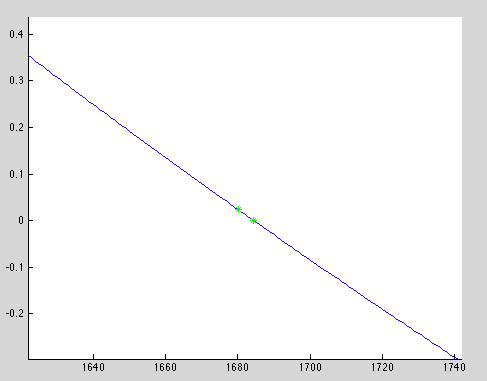
plot(C)

Results

A =

-3 1 0 0 0 0 0 0 0

2 -3 1 0 0 0 0 0 0

0 2 -3 1 0 0 0 0 0

0 0 2 -3 1 0 0 0 0

0 0 0 2 -3 1 0 0 0

0 0 0 0 2 -3 1 0 0

0 0 0 0 0 2 -3 1 0

0 0 0 0 0 0 2 -3 1

0 0 0 0 0 0 0 2 -3

B =

-160

-20

Concentration values =

79.9413

79.8240

79.5894

79.1202

78.1818

76.3050

72.5513

65.0440

50.0293

11.22

Write the following set of equations in matrix form:

50 = 5x_3 -7x_2
4x_2 + 7x_3 + 30 = 0
x_1 - 7x_3 = 40 - 3x_2 +5x_1

Use excel, MATLAB, or Mathcad to solve for the unkowns. In addition,
compute the transpose and the inverse of the coefficient matrix.

50 = 5x_3 -7x_2 + 0x_1
30 = - 7x_3 - 4x_2 + 0x_1
-40 = 7x_3 - 3x_2 +4x_1

Matlab Code:

A = [5 -7 0; -7 -4 0; 7 -3 4];

B = [50; 30; -40];

X = A\B;

%transpose

TransposeA = A.';

%inverse

inverseA = inv(A);

display(A)

display(B)

display(X)

display(TransposeA)

display(inverseA)

Results

A =

5 -7 0

-7 -4 0

7 -3 4

B =

-40

X =

-0.1449

-7.2464

-15.1812

TransposeA =

5 -7 7

-7 -4 -3

0 0 4

inverseA =

0.0580 -0.1014 0

-0.1014 -0.0725 0

-0.1775 0.1232 0.2500

X_1 = -0.1449

X_2 = -7.2464

X_3 = -15.1812

11.15

Of the following three sets of linear equations, identify the set(s) that you could not solve using an iterative method such as Gauss-seidel. Show using any number of iterations that is necessary that your solution does not converge. Clearly state your convergence criteria (how you know it is not converging).

set one

9x + 3y +z = 13

-6x + 8z =2

2x +5y -z = 6

set two

x +y +6z = 8

x+ 5y - z = 5

4x + 2y - 2z = 4

set three

-3x +4y +5z = 6

-2x +2y -4z = -3

2y -z = 1

Matlab code:

A = [9 3 1; -6 0 8; 2 5 -1];

B = [13; 2; 6];

solution1 = A \ B;

x = [0 0 0];

for ii = 1:100

x(1) = (B(1) - A(1,2) * x(2) - A(1,3) * x(3))/A(1,1);

x(2) = (B(2) - A(2,1) * x(1) - A(2,3) * x(3))/A(2,2);

x(3) = (B(3) - A(3,1) * x(1) - A(3,2) * x(2))/A(3,3);

end

display(solution1);

display(x);

%set two

A = [1 1 6; 1 5 -1; 4 2 -2];

B = [8;5;4];

solution2 =A\B;

x = [0 0 0];

for ii = 1:100

x(1) = (B(1) - A(1,2) * x(2) - A(1,3) * x(3))/A(1,1);

x(2) = (B(2) - A(2,1) * x(1) - A(2,3) * x(3))/A(2,2);

x(3) = (B(3) - A(3,1) * x(1) - A(3,2) * x(2))/A(3,3);

end

display(solution2);

display(x);

%set three

A = [-3 4 5; -2 2 -4; 0 2 -1];

B = [6; -3; 1];

solution3 =A\B;

x = [0 0 0];

for ii = 1:100

x(1) = (B(1) - A(1,2) * x(2) - A(1,3) * x(3))/A(1,1);

x(2) = (B(2) - A(2,1) * x(1) - A(2,3) * x(3))/A(2,2);

x(3) = (B(3) - A(3,1) * x(1) - A(3,2) * x(2))/A(3,3);

end

display(solution3);

display(x);

Results

solution1 =

1.0000e+00

x =

-Inf -Inf -Inf

solution2 =

x =

-2.3612e+101 5.5271e+100 -4.1696e+101

solution3 =

6.9565e-01

9.3478e-01

8.6957e-01

x =

-1.6803e+93 -3.1205e+93 -6.2411e+93

All 3 sets diverge

Saturday, April 21, 2012

10.25

Polynomial interpolation consists of determining the unique (n - 1)th-order polynomial that fits n data points. Such polynomials have the general form.

f(x) = P1x^n-1 + P2x^n-2 +... + Pn-1x +Pn (eq10.25)

where the p's are constant coefficients. A straightforward way for computing the coefficients is to generate n linear algebraic equations that we can solve simultaneously for the coefficients. Suppose that we want to determine the coefficients of the fourth-order polynomial f(x) = p1x^4 + p2x^3 +p3x^2 +p4x +p5 that passes through the following five points:(200,0.746),(250, .675), (300,.616), (400, .525) and (500, .457). Each of these pairs can be substituted into Eq. (P10.25) to yield a system of five equations with five unknowns (the p's). Use this approach to solve for the coefficients. In addition, determine and interpret the condition number.

Matlab code:

B = [ .746; .675; .616; .525; .457]

x = [200, 250, 300, 400, 500];

xx = [1,1,1,1,1];

A = [ x.^4 ;x.^3; x.^2 ;x.^1; xx]'

p = A\B

A * p

cond(A)

RESULTS

B =

7.4600e-01

6.7500e-01

6.1600e-01

5.2500e-01

4.5700e-01

A =

1.6000e+09 8.0000e+06 4.0000e+04 2.0000e+02 1.0000e+00

3.9062e+09 1.5625e+07 6.2500e+04 2.5000e+02 1.0000e+00

8.1000e+09 2.7000e+07 9.0000e+04 3.0000e+02 1.0000e+00

2.5600e+10 6.4000e+07 1.6000e+05 4.0000e+02 1.0000e+00

6.2500e+10 1.2500e+08 2.5000e+05 5.0000e+02 1.0000e+00

p =

1.3333e-12 P1

-4.5333e-09 P2

5.2967e-06 P3

-3.1737e-03 P4

1.2030e+00 P5

ans =

7.4600e-01

6.7500e-01

6.1600e-01

5.2500e-01

4.5700e-01

cond(A) =

1.1712e+13

A has a large condition number, meaning it is ill-formed, and there is a high potential for error

10.21

Consider vectors:
A = 2i - 3j + ak
B = bi + j - 4k
C = 3i + cj +2k

Vector A is perpendicular to B as well as to C. It is also known that B * C = 2. Use any method studied in this chapter to solve for the three unknowns, a, b, and c.

Matlab code:

% A * B = 0 ... 2bi -3j - 4ak = 0 ... 3j

% A * C = 0 ... 6i - 3cj + 2ak = 0... 6i

% B * C = 2 ... 3bi + cj - 8k = 2k... 10k

% a b c

A = [-4 2 0; 2 0 -3; 0 3 1]

b = [3; -6; 10]

x = A\b

display(A*x)

First take the dot products. Since A is perpendicular to B as well as to C we can say that they are orthogonal so their dot products are 0. We then pull the vectors 3j, 6i, and 8k from the dot products, leaving us with a b matrix of [3;6;10]. then solves for the unknowns, giving us A=0.5250, B=2.5500, and C=2.3500. We confirm the result by multiplying A and x, reproducing b

A =

-4 2 0

2 0 -3

0 3 1

b =

-6

x =

0.5250

2.5500

2.3500

ans =

3.0000

-6.0000

10.0000

10.15

(a)Determine the condition number for the following system using
the row-sum norm. Do not normalize the system.

A = [ 1 4 9 16 25;4 9 16 25 36; 9 16 25 36 49; 16 25 36 49 64;25 36 49 64 81]

How many digits of precision will be lost due to ill-conditioning?
(b)Repeat (a), but scale the matrix by making the maximum element in each
row equal to one.

Matlab Code:

A = [ 1 4 9 16 25;4 9 16 25 36; 9 16 25 36 49; 16 25 36 49 64;25 36 49 64 81]

%(a)

conditionA = cond(A)

significant = 10^(log10(cond(A)) - 7.2)

%(b)

b = [ 1/25 0 0 0 0;0 1/36 0 0 0;0 0 1/49 0 0;0 0 0 1/64 0;0 0 0 0 1/81];

A_scaled = b * A

conditionA_scaled = cond(A_scaled)

significant_scaled = 10^(log10(cond(A_scaled)) - 7.2)

RESULTS

A =

1 4 9 16 25

4 9 16 25 36

9 16 25 36 49

16 25 36 49 64

25 36 49 64 81

conditionA =

3.145210075463109e+17

significant =

1.984493397046558e+10

A_scaled =

0.040000000000000 0.160000000000000 0.360000000000000 0.640000000000000 1.000000000000000

0.111111111111111 0.250000000000000 0.444444444444444 0.694444444444444 1.000000000000000

0.183673469387755 0.326530612244898 0.510204081632653 0.734693877551020 1.000000000000000

0.250000000000000 0.390625000000000 0.562500000000000 0.765625000000000 1.000000000000000

0.308641975308642 0.444444444444444 0.604938271604938 0.790123456790123 1.000000000000000

conditionA_scaled =

9.237149093911445e+16

significant_scaled =

5.828247062861999e+09

These results show that both matrices are substantially ill-formed and there is a large loss of significance

10.8

The following system of equations is designed to determine concentrations (the c's in g/m^3) in a series of coupled reactors as a function of the amount of mass input to each reactor (the right-hand sides in g/day),

15c1 - 3c2 - c3 = 3300
-3c1 +18c2 - 6c3 = 1200
-4c1 - c2 + 12c3 = 2400

(a) Determine the matrix inverse(b) Use the inverse matrix to determine a solution(c) Determine how much the rate of mass input to reactor 3 must be increased to include a 10 g/m^3 rise in the concentration of reactor 1.(d)How much will the concentration in reactor 3 be reduced if the rate of mass input to reactors 1 and 2 is reduced by 700 and 350 g/day, respectively?

Matlab code:

%(a) Determine the matrix inverse

A = [15 -3 -1; -3 18 -6; -4 -1 12]

inversematrix = inv(A)

%(b) Use the inverse matrix to determine a solution

B = [3300; 1200; 2400]

x = inversematrix * B

OriginalB = A * x

%(c) Determine how much the rate of mass input to reactor

%3 must be increased to incduce a 10 g/m^3 rise in the concentration of

%reactor 1.

[x(1)+10; x(2); x(3)]

OriginalBplus10 = A * [x(1)+10; x(2); x(3)]

%(d)How much will the concentration in reactor 3 be reduced if the rate of

%mass input to reactors 1 and 2 is reduced by 700 and 350 g/day,

%respectively?

Bnew = [2600; 850; 2400]

newx = inversematrix * Bnew

newB = A * newx

diffx = x - newx

Results

(A)

A =

15 -3 -1

-3 18 -6

-4 -1 12

inversematrix =

0.072538860103627 0.012780656303972 0.012435233160622

0.020725388601036 0.060794473229706 0.032124352331606

0.025906735751295 0.009326424870466 0.090155440414508

(B)

B =

3300

1200

2400

x =

1.0e+02 *

2.845595854922280

2.184455958549223

3.130569948186529

OriginalB =

1.0e+03 *

3.299999999999999

1.200000000000001

2.400000000000000

ans =

1.0e+02 *

2.945595854922280

2.184455958549223

3.130569948186529

(C)

OriginalBplus10 =

1.0e+03 *

3.450000000000000

1.170000000000001

2.360000000000000

(D)

Bnew =

2600

850

2400

newx =

1.0e+02 *

2.293091537132988

1.826597582037997

2.916580310880829

newB =

1.0e+03 *

2.600000000000000

0.850000000000001

2.400000000000000

diffx =

55.250431778929169

35.785837651122620

21.398963730569960

10.5

Determine the total flops as a function of the number of equations n for the (a) decomposition, (b) forward-substitution, and (c) back-substitution phases of the LU decomposition version of Gauss elimination.

Decomposition
n^3/3 - n/3 or as n increases n^3/3 + O(n)

Forward-substitution
n^3/3 - n/3 + n^2 or as n increases n^3/3 + O(n^2)

Back-substitution
n^3/3 - n/3 + n^2 or as n increases n^3/3 + O(n^2)

Saturday, March 24, 2012

8.23

Many fields of engineering require accurate population estimates. For example, transportation engineers might find it necessary to determine separately the population growth trends of a city and adjacent suburb. The population of the urban area is declining with time according to.

Pu(t) = Pu, maxe^-kut + Pu, min

while the suburban population is growing , as in

Ps(t) = Ps, max/ 1+ [Ps, max/Po - 1] * e^-kst

where Pu, max, ku, Ps, max, Po, and ks = empirically derived parameters. Determine the time and corresponding values of Pu(t) and Ps(t) when the suburbs are 20% larger than the city. the parameter values are Pu,max = 75,000, ku = 0.45/yr, Pu, min = 100,000 people, Ps, max = 300,000 people, Po = 10000 people, ks = .08/yr. To obtain your solution,use (a) graphical, (b) false-position, and (c) modified secant methods.

Matlab Code:

Pumax = 75000;

ku = 0.045;

Pumin = 100000;

Psmax = 300000;

Po = 10000;

ks = .08;

t = 0:100;

pu = @(t) Pumax * exp(-ku * t) + Pumin;%city

ps = @(t) Psmax ./ ( 1 + (Psmax /Po - 1) * exp(-ks * t));%suburbs

p = @(t) 1.2 * pu(t) - ps(t); %find zero of this to find intersection of pu and ps

%(a)graphically

hold on

plot(t,pu(t));

plot(t, ps(t) , 'r');

plot(t,p(t),'g');

%(b)false-position

t_l = 40;

t_u = 20;

for i = 1:1:8

% if f(x_l) * f(x_u) < 0 the signs should be opposite

t_r = t_u - ((p(t_u) * (t_l - t_u)) / (p(t_l) - p(t_u))); % x_r is our estimated root

if (p(t_l) * p(t_r) < 0)

t_u = t_r;

else

%(p(t_l) * p(t_r) > 0)

t_l = t_r;

%(p(t_l) * p(t_r) == 0)

end

plot(t_r ,p(t_r),'y*')

end

%(c)

t = 40;

delta = .01;

%Modified secant method

for i = 1:23

t_new = t - (delta * t * p(t)) ./ (p(t + delta*t) - p(t));

t = t_new;

plot(t,p(t), 'k*')

end

hold off

The red line shows the suburbs, the blue shows the city, and the green line is the equation we came up with to find the desired intersection(where the suburbs are 20% larger than the city). This graph looks to be giving an answer of about 40 years. It's hard to see the results of the other two methods, so we'll zoom in a bit.

The yellow dot is the result of the false position method, and the black is the result of the modified secant method both approximating the zero. The results of these two methods are as follows, t being the modified secant and t_r being the false position

EDU>> t

t =

39.606797739143595

EDU>> t_r

t_r =

39.606797739143595

EDU>> p(t)

ans =

-2.910383045673370e-11

EDU>> p(t_r)

ans =

-2.910383045673370e-11

They are identical results to the degree of accuracy matlab will display, and when plugged back in to the equation, they are negligibly far from 0, thus they confirm each other quite well

8.17

Catenary cable is one that is hung between two points not in the same vertical line. As depicted in Fig. P8.17a, it is subject to no loads other than its own weight. Thus, its weight (N/m) acts as a uniform load per unit length along the cable. A free-body diagram of a section AB is depicted in Fig. P8.17b, where T_a and t_b are there tension forces at the end. Based on horizontal and vertical force balances, the following differential equation model of the cable can be derived:

d^2y/dx^2 = w/ T_a * sqrt(1 + (dy/dx)^2)

Calculus can be employed to solve this equation for the height y of the
cable as a function of distance x,

y = T_a/w * cosh(w/T_a *x) + y_0 - T_A/w

where the hyperbolic cosine can be computed by

cosh x = 1/2(e^x + e^-x)

Use a numerical method to calculate a value for the parameter T_A
given values for the parameters w = 12 and y_0 = 6, such that the cable
has a height of y = 15 at x = 50.

Figure 8.17:

Matlab code:

y = 15; %height of the cable at a point

x = 50;% point of tension

T_a = 1000:2000; % Tensor force

w = 12; %angular velocity tensor

y_o = 6;

f = @(T_a) ((T_a ./ w) .* cosh(w ./ T_a * x) + y_o - T_a ./ w) - y;

%f = @(T_a) -T_a ./12 + 1/12 * T_a .* cosh(600 ./T_a) - 9;

hold on

plot( T_a, f(T_a))

T_a = 1600.;

delta = .001;

%Modified secant method

for i = 1:23

T_a_new = T_a - (delta * T_a * f(T_a)) ./ (f(T_a + delta*T_a) - f(T_a));

T_a = T_a_new;

plot(T_a,f(T_a), 'g*')

end

hold off

This produces

with the results of the modified secant method shown in green. To verify this answer, we used wolfram alpha to solve the equation, and it returned 1684.37. Matlab gives us

EDU>> T_a

T_a =

1.6844e+03

EDU>> f(T_a)

ans =

-2.8422e-14

from the modified secant, which simplified is T_a=1684.4 and f(T_a)=essentially 0, confirming the result.

8.14

In structural engineering, the secant formula defines the force per unit
area, P / A, that causes a maximum stress sigma_m in a column of given
slenderness ratio L/K:

P/A = sigma_m / 1 + (ec/ k^2) sec[.5* sqrt( P/(EA)(L/k)]

where ec/ k^2 = the eccentricity ratio an E = the modulus of elasticity.
If for a steel beam, E = 200,000 MPa, ec/k^2 = .4, and sigma_m = 250 MPa,
compute P/ A for L / k = 50. Recall that sec x = 1/ cos(x).
Matlab Code:

E = 200000;

eck = .4;

sigma_m = 250;

LK = 50;

PA = 0:300;

%PA = sigma_m / 1 + (eck) * sec(.5 * sqrt( P/(EA) * (LK)));

f = @(PA) (sigma_m / 1 + (eck) * sec(.5 * sqrt( (PA * 1/E )* (LK)))) - PA;

hold on

plot(PA,f(PA))

PA = 250;

delta = .0001;

%Modified secant method

for i = 1:40

PA_new = PA - (delta * PA * f(PA)) ./ (f(PA + delta*PA) - f(PA));

PA = PA_new;

plot(PA,f(PA), 'r*')

end

hold off

This produces

which makes sense given that the equation is 250 divided by a value close to 1. The actual zero lies at 250.4032 as proven by plugging the result of applying the modified secant method (the red dot) back into the equation (graphed in blue) as such:

EDU>> PA

PA =

250.4032

EDU>> f(PA)

ans =

8.9

The volume V of liquid in a spherical tank of radius r is related to the depth h of the liquid by

V = pi * h .^2 *(3*r - h) ./3

Determine h given r = 1 m and V= .5m^3.
Matlab code:

h = -30:30;

r = 1;

V = .5; % m .^3

f = @(h) (pi .* h .^2 .*(3*r - h) ./ 3) - V;

hold on

plot(h , f(h))

h = .43;

delta = .0001;

%Modified secant method

for i = 1:40

h_new = h - (delta * h * f(h)) ./ (f(h + delta*h) - f(h));

h = h_new;

plot(h,h, 'r*')

end

hold off

This produces

The modified secant method was used to pinpoint the solution at .4311

7.19

In control systems analysis, transfer functions are developed that mathematically relate the dynamics of a system's input to its output. A transfer function for robotic positioning system is given by

G(s) = C(s)/N(s) = s^3 +12.5 *s^2 + 50.5 *s +66/ s^4 + 19*s^3 +122*s^2 +296 * s +192

where G(s) = system gain, C(s) = system output, N(s) = system input, and s = Laplace transform complex frequency. Use a numerical technique to find the roots of the numerator and denominator and factor these into the form

G(s) = (s + a_1) (s + a_2) (s + a_3) / (s + b_1)(s + b_2)(s + b_3)(s + b_4)

where a_i and b_i = the roots of the numerator and denominator, respectively.

%roots(s^3 +12.5 *s^2 + 50.5 *s +66)

x = roots([1 12.5 50.5 66]);

%roots(s^4 + 19*s^3 +122*s^2 +296 * s +192)

y = roots([1 19 122 296 192]);

This results in

EDU>> x

x =

-5.5000
-4.0000
-3.0000

EDU>> y

y =

-8.0000
-6.0000
-4.0000
-1.0000

And so,

G(s) = (s + 5.5) (s + 4) (s + 3) / (s + 8) (s + 6) (s + 4) (s + 1)

7.17

When trying to find the acidity of a solution of magnesium hydroxide in hydrochloric acid, we obtain the following equation.

A(x) = x^3 + 3.5x^2 - 40

where x is the hydronium ion concentration. Find the hydronium ion concentration for a saturated solution (acidity equals zero) using two different methods in MATLAB.

x = [-2:.01:5];

A = [1 3.5 0 -40];

A2 = @(X) x .^3 + 3.5 * x .^2 - 40;

hold on

plot(x, polyval(A,[x]))

plot(x, A2(x),'r')

%plot(x, polyval(polyder(A),[x]),'r')

x_0 = 2;

k = polyder(A);

%Newton- Raphson method

for ii =1:23

plot(x_0 ,polyval(A,x_0),'*g')

x = x_0 - (polyval(A,x_0) ./ polyval(k,x_0));

x_0 = x;

end

hold off

The polyval function allows one to graph the polynomial and find the zero by simply evaluating it, and the newton-raphson method confirms the zero by converging to an x value of 2.5676, which when plugged into the equation gives us a value of zero

EDU>> x_0

x_0 =

2.5676

EDU>> polyval(A,x_0)

ans =