8.17

Catenary cable is one that is hung between two points not in the same vertical line. As depicted in Fig. P8.17a, it is subject to no loads other than its own weight. Thus, its weight (N/m) acts as a uniform load per unit length along the cable. A free-body diagram of a section AB is depicted in Fig. P8.17b, where T_a and t_b are there tension forces at the end. Based on horizontal and vertical force balances, the following differential equation model of the cable can be derived:

d^2y/dx^2 = w/ T_a * sqrt(1 + (dy/dx)^2)

Calculus can be employed to solve this equation for the height y of the
cable as a function of distance x,

y = T_a/w * cosh(w/T_a *x) + y_0 - T_A/w

where the hyperbolic cosine can be computed by

cosh x = 1/2(e^x + e^-x)

Use a numerical method to calculate a value for the parameter T_A
given values for the parameters w = 12 and y_0 = 6, such that the cable
has a height of y = 15 at x = 50.


Figure 8.17:

Matlab code:

y = 15; %height of the cable at a point

x = 50;% point of tension

T_a = 1000:2000; % Tensor force

w = 12; %angular velocity tensor

y_o = 6;

f = @(T_a)  ((T_a ./ w) .* cosh(w ./ T_a * x) + y_o - T_a ./ w) - y;

%f = @(T_a) -T_a ./12 + 1/12 * T_a .* cosh(600 ./T_a) - 9;

hold on

plot( T_a, f(T_a))

T_a = 1600.;

delta = .001;

%Modified secant method

for i = 1:23

    T_a_new = T_a - (delta * T_a * f(T_a)) ./ (f(T_a + delta*T_a) - f(T_a));

    T_a = T_a_new;

    

    plot(T_a,f(T_a), 'g*')

end

hold off

This produces 

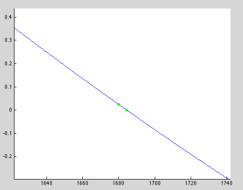
with the results of the modified secant method shown in green.  To verify this answer, we used wolfram alpha to solve the equation, and it returned 1684.37.  Matlab gives us 

EDU>> T_a

T_a =

   1.6844e+03

EDU>> f(T_a)

ans =

  -2.8422e-14

from the modified secant, which simplified is T_a=1684.4 and f(T_a)=essentially 0, confirming the result.