8.23

Many fields of engineering require accurate population estimates. For example, transportation engineers might find it necessary to determine separately the population growth trends of a city and adjacent suburb. The population of the urban area is declining with time according to.

Pu(t) = Pu, maxe^-kut + Pu, min

while the suburban population is growing , as in

Ps(t) = Ps, max/ 1+ [Ps, max/Po - 1] * e^-kst

where Pu, max, ku, Ps, max, Po, and ks = empirically derived parameters. Determine the time and corresponding values of Pu(t) and Ps(t) when the suburbs are 20% larger than the city. the parameter values are Pu,max = 75,000, ku = 0.45/yr, Pu, min = 100,000 people, Ps, max = 300,000 people, Po = 10000 people, ks = .08/yr. To obtain your solution,use (a) graphical, (b) false-position, and (c) modified secant methods.


Matlab Code:

Pumax = 75000;

ku = 0.045;

Pumin = 100000; 

Psmax = 300000; 

Po = 10000; 

ks = .08;

t = 0:100;

pu = @(t) Pumax * exp(-ku * t) + Pumin;%city

ps = @(t) Psmax ./ ( 1 + (Psmax /Po - 1) * exp(-ks * t));%suburbs

p = @(t) 1.2 * pu(t) - ps(t); %find zero of this to find intersection of pu and ps

%(a)graphically

hold on

plot(t,pu(t));

plot(t, ps(t) , 'r');

plot(t,p(t),'g');

%(b)false-position

t_l = 40;

t_u = 20;

for i = 1:1:8

   % if  f(x_l) * f(x_u) < 0  the signs should be opposite

   

  t_r = t_u - ((p(t_u) * (t_l - t_u)) / (p(t_l) - p(t_u))); % x_r is our estimated root

  

   if (p(t_l) * p(t_r) < 0)

       t_u = t_r;

   else

   %(p(t_l) * p(t_r) > 0)      

          t_l = t_r;   

   %(p(t_l) * p(t_r) == 0)   

   end

        

   plot(t_r ,p(t_r),'y*')

end

%(c)

t = 40;

delta = .01;

%Modified secant method

for i = 1:23

    t_new = t - (delta * t * p(t)) ./ (p(t + delta*t) - p(t));

    t = t_new;

    plot(t,p(t), 'k*')

end

hold off

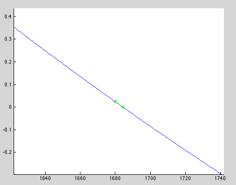
The red line shows the suburbs, the blue shows the city, and the green line is the equation we came up with to find the desired intersection(where the suburbs are 20% larger than the city). This graph looks to be giving an answer of about 40 years. It's hard to see the results of the other two methods, so we'll zoom in a bit.

The yellow dot is the result of the false position method, and the black is the result of the modified secant method both approximating the zero. The results of these two methods are as follows, t being the modified secant and t_r being the false position

EDU>> t

t =

  39.606797739143595

EDU>> t_r

t_r =

  39.606797739143595

EDU>> p(t)

ans =

    -2.910383045673370e-11

EDU>> p(t_r)

ans =

    -2.910383045673370e-11

They are identical results to the degree of accuracy matlab will display, and when plugged back in to the equation, they are negligibly far from 0, thus they confirm each other quite well

8.17

Catenary cable is one that is hung between two points not in the same vertical line. As depicted in Fig. P8.17a, it is subject to no loads other than its own weight. Thus, its weight (N/m) acts as a uniform load per unit length along the cable. A free-body diagram of a section AB is depicted in Fig. P8.17b, where T_a and t_b are there tension forces at the end. Based on horizontal and vertical force balances, the following differential equation model of the cable can be derived:

d^2y/dx^2 = w/ T_a * sqrt(1 + (dy/dx)^2)

Calculus can be employed to solve this equation for the height y of the
cable as a function of distance x,

y = T_a/w * cosh(w/T_a *x) + y_0 - T_A/w

where the hyperbolic cosine can be computed by

cosh x = 1/2(e^x + e^-x)

Use a numerical method to calculate a value for the parameter T_A
given values for the parameters w = 12 and y_0 = 6, such that the cable
has a height of y = 15 at x = 50.


Figure 8.17:

Matlab code:

y = 15; %height of the cable at a point

x = 50;% point of tension

T_a = 1000:2000; % Tensor force

w = 12; %angular velocity tensor

y_o = 6;

f = @(T_a)  ((T_a ./ w) .* cosh(w ./ T_a * x) + y_o - T_a ./ w) - y;

%f = @(T_a) -T_a ./12 + 1/12 * T_a .* cosh(600 ./T_a) - 9;

hold on

plot( T_a, f(T_a))

T_a = 1600.;

delta = .001;

%Modified secant method

for i = 1:23

    T_a_new = T_a - (delta * T_a * f(T_a)) ./ (f(T_a + delta*T_a) - f(T_a));

    T_a = T_a_new;

    

    plot(T_a,f(T_a), 'g*')

end

hold off

This produces 

with the results of the modified secant method shown in green.  To verify this answer, we used wolfram alpha to solve the equation, and it returned 1684.37.  Matlab gives us 

EDU>> T_a

T_a =

   1.6844e+03

EDU>> f(T_a)

ans =

  -2.8422e-14

from the modified secant, which simplified is T_a=1684.4 and f(T_a)=essentially 0, confirming the result.

8.14

In structural engineering, the secant formula defines the force per unit
area, P / A, that causes a maximum stress sigma_m in a column of given
slenderness ratio L/K:

P/A = sigma_m / 1 + (ec/ k^2) sec[.5* sqrt( P/(EA)(L/k)]
  
 where ec/ k^2 = the eccentricity ratio an E = the modulus of elasticity.
If for a steel beam, E = 200,000 MPa, ec/k^2 = .4, and sigma_m = 250 MPa,
 compute P/ A for L / k = 50. Recall that sec x = 1/ cos(x).
Matlab Code:

E = 200000; 

eck = .4;

sigma_m = 250; 

LK = 50;

PA = 0:300;

%PA = sigma_m / 1 + (eck) * sec(.5 * sqrt( P/(EA) * (LK))); 

f = @(PA) (sigma_m / 1 + (eck) * sec(.5 * sqrt( (PA * 1/E )* (LK)))) - PA; 

hold on

plot(PA,f(PA))

PA = 250;

delta = .0001;

%Modified secant method

for i = 1:40

    PA_new = PA - (delta * PA * f(PA)) ./ (f(PA + delta*PA) - f(PA));

    PA = PA_new;

    

    plot(PA,f(PA), 'r*')

end

hold off

This produces

which makes sense given that the equation is 250 divided by a value close to 1. The actual zero lies at 250.4032 as proven by plugging the result of applying the modified secant method (the red dot) back into the equation (graphed in blue) as such:

EDU>> PA

PA =

  250.4032

EDU>> f(PA)

ans =

     0

8.9

The volume V of liquid in a spherical tank of radius r is related to the depth h of the liquid by

V = pi * h .^2 *(3*r - h) ./3

Determine h given r = 1 m and V= .5m^3.
Matlab code:

h = -30:30;

r = 1;

V = .5; % m .^3

f = @(h) (pi .* h .^2 .*(3*r - h) ./ 3) - V;

hold on

plot(h , f(h))

h = .43;

delta = .0001;

%Modified secant method

for i = 1:40

    h_new = h - (delta * h * f(h)) ./ (f(h + delta*h) - f(h));

    h = h_new;

    

    plot(h,h, 'r*')

end

hold off

This produces 

The modified secant method was used to pinpoint the solution at .4311

7.19

In control systems analysis, transfer functions are developed that mathematically relate the dynamics of a system's input to its output. A transfer function for robotic positioning system is given by

G(s) = C(s)/N(s) = s^3 +12.5 *s^2 + 50.5 *s +66/ s^4 + 19*s^3 +122*s^2 +296 * s +192

where G(s) = system gain, C(s) = system output, N(s) = system input, and s = Laplace transform complex frequency. Use a numerical technique to find the roots of the numerator and denominator and factor these into the form

G(s) = (s + a_1) (s + a_2) (s + a_3) / (s + b_1)(s + b_2)(s + b_3)(s + b_4)

where a_i and b_i = the roots of the numerator and denominator, respectively.

%roots(s^3 +12.5 *s^2 + 50.5 *s +66)

x = roots([1 12.5 50.5 66]);

%roots(s^4 + 19*s^3 +122*s^2 +296 * s +192)

y = roots([1 19 122 296 192]);

This results in 

EDU>> x


x =


   -5.5000
   -4.0000
   -3.0000


EDU>> y


y =


   -8.0000
   -6.0000
   -4.0000
   -1.0000


And so, 



G(s) =   (s + 5.5)  (s + 4) (s + 3)  / (s + 8)  (s + 6)  (s + 4)  (s + 1)

7.17

When trying to find the acidity of a solution of magnesium hydroxide in hydrochloric acid, we obtain the following equation.

A(x) = x^3 + 3.5x^2 - 40

where x is the hydronium ion concentration. Find the hydronium ion concentration for a saturated solution (acidity equals zero) using two different methods in MATLAB.

x = [-2:.01:5];

A = [1 3.5  0 -40];

A2 = @(X) x .^3 + 3.5 * x .^2 - 40;

hold on

plot(x, polyval(A,[x]))

plot(x, A2(x),'r')

%plot(x, polyval(polyder(A),[x]),'r')

x_0 = 2;

k = polyder(A);

%Newton- Raphson method

for ii =1:23

     plot(x_0 ,polyval(A,x_0),'*g')

    x = x_0 - (polyval(A,x_0) ./ polyval(k,x_0));

    

    x_0 = x;  

end

hold off

The polyval function allows one to graph the polynomial and find the zero by simply evaluating it, and the newton-raphson method confirms the zero by converging to an x value of 2.5676, which when plugged into the equation gives us a value of zero

EDU>> x_0

x_0 =

    2.5676

EDU>> polyval(A,x_0)

ans =

     0

6.31

The Manning equation can be written for a rectangular open channel as

Q = ((sqrt(S) * (B*H)^(5/3))/(n*(B +2*H)^(2/3)));

where Q = flow [m^3/s], S = slope [m/m], H = depth[m],
and n = the manning roughness coefficient. Develop a fixed-point iteration
scheme to solve this equation for H given Q = 5, S = 0.0002, B = 20 , and
n = 0.03. Prove that your scheme converges for all initial guesses greater
than or equal to zero.


Matlab code:

H = 0:.0001:4;

Q = 5;

S = 0.0002;

B = 20;

n = 0.03;

hold on

%Q = @(H) ((sqrt(S) * (B*H) .^(5/3))/(n*(B +2*H) .^(2/3)));  %Original Q

f = @(H) (sqrt(S)*(B*H).^(5/3) ./ (n*(B+2*H).^(2/3)))-Q;        %Rearranged

plot(H,f(H))

g = @(H) (((Q * (n*(B +2*H) .^(2/3))) ./ (sqrt(S))) .^(3/5))/B ;  %arranged to solve for H

H = 1;

for ii = 1:10,

H = g(H);

plot(H,f(H),'*g')

end

EDU>> H

H =

    0.7023

EDU>> f(H)

ans =

     0

6.28

The polynomial f(x) = 0.0074*x^4 - .284*x^3 + 3.355x^2 - 12.183*x +5 has areal root between 15 and 20. Apply the Newton- Raphson method to this function using an initial guess of x_0 = 16.15. Explain your results. 


Matlab code

p = [0.0074 -.284 3.355 -12.183 5];

x_i = [15:0.001:20];

f = @(x) 0.0074*x .^4 - .284*x .^3 + 3.355 *x .^2 - 12.183*x + 5;

hold on

plot(x_i, polyval(p,x_i))

plot(x_i, polyval(polyder(p),x_i), 'r')

%x_0 = 16.5;%bad

x_0 = 18;%good

k = polyder(p);

for ii =1:100

     plot(x_0 ,f(x_0),'*g')

    x = x_0 - (polyval(p,x_0) ./ polyval(k,x_0));

    x_0 = x;

end

Results:

Using the specified initial guess of 16.5, Newton-Raphson diverges badly

Using an initial guess of 18, a little farther through the test range, it converges much more nicely

x =

   18.8948

EDU>> f(x)

ans =

  -5.6843e-14

The real root is at 18.8948. Plugging it back into the equation results in -5.6843e-14, which is negligible from 0

6.18

A mass balance for a pollutant in a well-mixed lake can be written as

V * dc/dt = W - Q*c - k * V * sqrt(c)

Given the parameter values V = 1 * 10^6 m^3 , Q = 1 * 10^5 * m^3/yr,W = 1 * 10^6 g/yr, and k = .25 m^0.5/g^0.5/yr, use the modified secant method to solve for the steady-state concentration. Employ an initial guess of c = 4 g/m^3 and delta = .5. Perform three iterations and determine the percent relative error after the third iteration.

Matlab Code:

V = 1.0 * 10^6; % m^3 

Q = 1.0 * 10^5 ; % m^3/yr,

W = 1.0 * 10^6 ; %g/yr

k = .25; % m^0.5/g^0.5/yr,

c = -20:20;

f = @(c) W - Q .* c - k * V * sqrt(c);

hold on

plot(c, f(c))

c = 4; % g/m^3

delta = .05; 

for ii = 1:5

    plot(c, f(c), '*r')

    

    c_new = c - (delta * c * f(c))/(f(c + delta * c) - f(c));

    c = c_new;

end

hold off

percent_relative_error = ((c_new - c)/c_new) *100

The resulting percent relative error was 0

6.15

Determine the roots of the following simultaneous nonlinear equations using 

(a) fixed-point iteration and (b) the newton-Raphson method.

 y = -x^2 + x + 0.75

 y + 5xy =x^2

Employ initial guesses of x = y = 1.2 and discuss the results.

x = -1:-.25;

y = -1:5;

fx = @(x,y) y + x .^2  - .75; %solved for y

fy = @(x,y) (-5 .* x .* y) + x .^2 ;%solved for y

%fy = @(x,y) (-5 .* y + 1) .* x ;%solved for y

%fy = @(x,y) -x .^2  + x + .75; %solved for y

%fx = @(x,y) sqrt((5 .* x .* y) + y) ;%solved for y

%fx = @(x,y) sqrt(-y + x  - .75); %solved for y

%fy = @(x,y) (x .^2)/ (1 + 5*x) ;%solved for y

hold on

plot (fy(x,y))

plot (fx(x,y))

% newton-raphson for systems of non-linear equations

u = @(x,y) - x .^2 + x + .75 - y; % u derivitation by parts

v = @(x,y) y + 5 .* x .* y - x .^2;%v derivitation by parts

dudx =@(x,y) -2 * x + 1;

dudy = @(x,y) -1;

dvdx = @(x,y) 5*y - 2*x;

dvdy = @(x,y) 1+ 5*x;

%y1 = fy(x,y); first iteration of y

%x1 = fx(x,y);first iteration of x

%y2 = fy(x1,y1); second iteration of y

%x2 = fx(x1,y1);second iteration of x

x = 1.2;

y = .2;

for ii = 1:3

   

    ny = fy(x,y);

    nx = fx(x,y);

    

   y = ny;

   x = nx;

   plot(x,y,'*r') 

end

%guess

x = 4; y = 0;

denom = ((dudx(x,y) * dvdy(x,y)) - (dudy(x,y) * dvdx(x,y)));

for ii = 0:15

denominator = denom + ( denom == 0) ;

x_1 = x - (((u(x,y) * dvdy(x,y)) - (v(x,y) * dudy(x,y))) / denominator);

y_1 = y - (((v(x,y) * dudx(x,y)) - (u(x,y) * dvdx(x,y))) / denominator);

x = x_1;

y = y_1;

plot( x_1 , y_1, '*g')

end

hold off

When running the fixed point at the initial guesses specified, it diverges very quickly, so we chose to start the y at .2 instead because it is closer. Nevertheless, even after bringing the initial guess closer, it diverges after 4 iterations. The newton Raphson method was also rather inaccurate at first, but x=4, y=0 seemed to get quite close, though still not quite there.

6.5

Employ the newton-Raphson method to determine a real root for f(x) = -2 +6x - 4x^2 +.5x^3 using initial guesses of (a) 4.2 and (b) 4.43. Discuss and use graphical and analytical methods to explain any peculiarities in your results.


Matlab Code:

x = 0:.001:5;

f = @(x) -2 +6 * x - 4 * x .^2 + 0.5 * x .^3;

hold on

plot (x,f(x))

%(a) Newton-Raphson method (three iterations, x_0 = 4.2).

df = @(x) 6 - 2 * 4 * x + 3 * 0.5 * x .^2; 

ax = 4.2;

for n = 1:1:23

ax_n = ax - f(ax) ./ df(ax);

ax = ax_n;

end

plot (ax_n, x, 'k')

error_approximatea = (ax_n - ax) ./ ax_n;

%(b) Newton-Raphson method (three iterations, x_0 = 4.43).

bx = 4.43;

for n = 1:1:23

bx_n = bx - f(bx) ./ df(bx);

bx = bx_n;

end

plot (bx_n, x, 'r')

error_approximateb = (bx_n - bx) ./ bx_n;

Red is the approximation to the real root 4.43
Black is the approximation to the real root 4.2
Blue is f(x) = -2 +6x - 4x^2 +.5x^3



EDU>> ax_n


ax_n =


    0.4746


EDU>> bx_n


bx_n =


    0.4740


EDU>> error_approximatea


error_approximatea =


     0


EDU>> error_approximateb


error_approximateb =


     0